Case Study: Rapid Conversion of a Technical Paper to a Mathematical Model
Introduction
A technical paper, in PDF form, containing
an algorithm with over sixty linear, nonlinear and integral equations is
converted to a mathematical model in TK Solver and subsequently linked to Excel
and a web application. The math model
was completed in one day and the links and refinements to the interface were
completed on day two.
The Model Building Process
The technical paper was ESDU Data Item
85007, entitled “Contact Phenomena III:
Calculation of Individual Stress Components in Concentrated Elastic
Contacts Under Combined Normal and Tangential Loading.” It was made available in PDF form.
The PDF file was briefly reviewed and it
was noted that two complete examples were provided within the document, either
of which could be used to verify a computerized version of the formulas and
calculations.
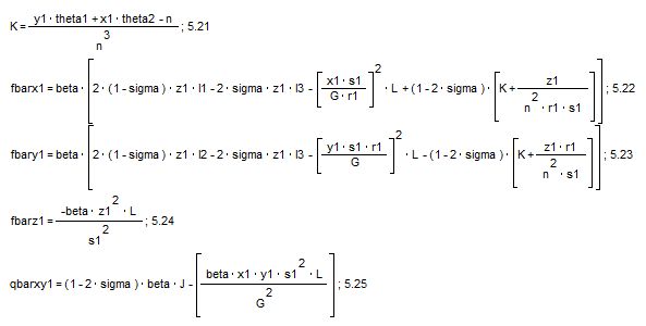
The formulas were entered into TK
Solver. Here is a sample of some of the
formulas, in TK’s MathLook View including the equation numbers from the paper:
There are 57 such equations in the math model, in addition to
several functions which were added to perform tasks such as generate
plots. These will be discussed in more
detail later.
The variables in the equations are
automatically summarized on TK’s variable sheet, including descriptions and
units. Here is a portion of the variable
sheet, with the inputs grouped at the top.
The model also includes many auxiliary
variables used by the ESDU algorithm. Those variables are grouped together on the
variable sheet. During the testing of
the model, it was very useful to be able to verify that each intermediate value
was computed as specified by the paper.
Here is a portion of that listing.
The calculations required three numerical
integrations. Fortunately, TK Solver
includes built-in functions for those calculations. Here are the integrands.
The limits of the integrals were determined from the solution
of a sixth order polynomial. It was
necessary to find all the roots and then use the largest real root in the upper
limit of integration. TK Solver includes
a root finder that was perfect for the task, based on Bairstow’s algorithm for
finding real and complex roots of nth-order polynomials. A loop was added to select the best one for
this application. TK’s unique capability
to mix rule-based equation solving with calls to procedural subroutines was a
time-saver.
Here is the procedure that sets up the polynomial, solves it with a call to the Bairstow function and then picks the best solution for the application.
The model takes a fraction of a second to
solve and the solutions verify the values from the example in the paper.
Interfacing with Excel
The TK file was linked to an Excel
spreadsheet, as shown below. There are
several advantages to this. The
underlying formulas can be hidden. The
interface can be customized. The TK
model can be used as a function within a larger spreadsheet application. The spreadsheet and model can be packaged together
and shared with anyone.
The spreadsheet dynamically updates as the
inputs are changed. The plots were added
by taking advantage of TK’s powerful “List Solve” feature to repeatedly solve
the equations over a range of inputs for one of the variables.
Interfacing with the Web
The TK Solver model was also processed
using a UTS tool called Galaxy, which automatically builds a browser interface
for a web-based application. Again, the
variables displayed in the browser interface are dynamically linked to the
model.
Odds and Ends
There are a number of additional features
of TK Solver that make it an excellent tool for such applications.
Units management is one TK’s strengths. In
this application, unit conversions are available for all the inputs and
outputs. You can globally swap between
US and SI units or mix and match as you like.
This feature carries through to the Excel and Web interfaces as well.
Table and plot generation is another asset. Any
mathematical model built in TK Solver can be enhanced without any additional
programming required. As shown, the
effects of varying the friction angle are plotted and automatically updated as
other variables change. Even the
locations of the plot annotations dynamically change.
Backsolving
is perhaps TK Solver’s most valuable feature.
Backsolving allows users to input a desired value for one or more
outputs and solve for the required inputs.
One example for this model would be to input a stress value and have TK
determine the required friction angle or contact dimension. Here is one such example. Note that fy, the component stress with the
maximum absolute value, has been input and the contact length, a, has been solved.
In this way, a single TK Solver model
actually solves much more than the initial intent of the technical paper, with
no additional programming required.
In summary, a technical paper containing
dozens of pages of equations is now accompanied by a mathematical model that
the reader can immediately use to solve any related problems. With much more functionality than FORTRAN or
BASIC translations of the formulas could provide, the TK Solver model gives the
reader a dynamic way of turning a complex document into a handful of variables
that are easily understand and manipulated.
Best of all, the entire process only required a couple days.


